Bayesian A/B testing with confidence

UPDATE (12/30/2015): In response to a comment by Niels Oppermann, I have added derivations of the expected difference \(p_B-p_A\) in addition to the expected gain \(\mathrm{max}\left(p_B-p_A, 0\right)\) (i.e. the difference when \(p_B>p_A\)).

I have been developing the A/B testing procedure that I want to use in an upcoming experiment at work. Generally speaking I'm on team Bayes when it comes to statistical matters, and that's the approach that I will take in this case as well. In this (long) post I'll outline a method for Bayesian A/B testing that is largely built on some excellent blog posts by Evan Miller, Chris Stuccio, and David Robinson. In this post I'll summarize the results of Miller and Stuccio, ending up with a decision function for A/B testing based on the gain expected from making the change that is under consideration. I go a bit further than the referenced posts by deriving a measure of uncertainty in the expected gain that can be used to determine when a result is significant and overcome the "peeking" problem discussed in Robinson's post. Lastly I calculate the expected difference between the two procedures under test (as opposed to the gain which is the difference but only when the new procedure is better). Throughout I present some simulated examples to give a sense of the impact of the different parameters in the model and to illustrate some aspects of the model that one should be aware of.

The basic model

In an A/B test, one has two different procedures (i.e. treatments) under consideration and would like to know which one produces the best results. For example, an e-commerce company might have a couple of different web site layouts that they are considering and would like to know which one has the best click through rate to a product page. An experiment is run where two groups are selected at random from the overall population. The control group A uses the standard procedure and the test group B uses the new procedure. At the end of the experiment the data is analyzed to decide whether the outcome for group B was better (or worse, or the same) than the outcome for group A.

In the simplest case, which I consider here, the outcome is binary, e.g. either a customer clicked through to a product page or they didn't. In this case, the most natural choice for the likelihood, i.e. the probability that a number of positive outcomes k is observed from a total of n trials with probability of success p per trial, is the Binomial distribution

\begin{equation}P(k|n,p)=\mathrm{Binomial}(k;n,p)=\left(\begin{array}{c}n\\k\end{array}\right)p^{k}\left(1-p\right)^{n-k}.\end{equation}

Of course n and k can be measured experimentally, but p must be inferred. It's time for Bayes' theorem (the important bit of it anyway)

\begin{equation}P\left(p|k,n\right)\propto P(k|n,p)P(p)\end{equation}

where \(P(p)\) describes any prior knowledge about p. A convenient choice of prior distribution is the Beta distribution which is conjugate to the Binomial distribution

\begin{equation}P(p)=\mathrm{Beta}(p;\alpha,\beta)=\frac{p^{\alpha-1}(1-p)^{\beta-1}}{\mathrm{B}(\alpha,\beta)}\end{equation}

where \(\alpha\) and \(\beta\) are parameters of the Beta distribution and \(\mathrm{B}(\alpha,\beta)\) is the Beta function. The parameters \(\alpha\) and \(\beta\) can be set empirically from historical data, using hierarchical modeling, or chosen manually. For instance, a uniform prior on the interval [0,1] can be chosen by setting \(\alpha=1\) and \(\beta=1\).

A Binomial likelihood and Beta prior leads to a posterior distribution that is also Beta distributed

\begin{equation}P\left(p|k,n\right)=p^{k+\alpha-1}\left(1-p\right)^{n-k+\beta-1}=\mathrm{Beta}(p;\alpha+k,n-k+\beta)=\mathrm{Beta}(p;\alpha',\beta')\end{equation}

where \(\alpha'=\alpha+k\) is the prior parameter \(\alpha\) plus the number of successful trials and \(\beta'=n-k+\beta\) is the prior parameter \(\beta\) plus the number of failed trials.

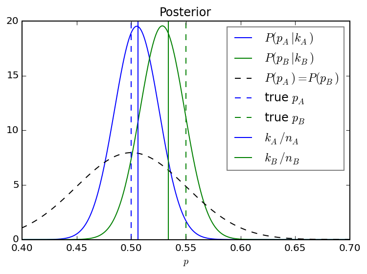
The figure below shows the posterior distributions for \(p_{A}\) and \(p_{B}\) for a simulated data set with \(n=500\) observations. I have chosen a true \(p_{A}\) of 0.5, a true \(p_{B}\) of 0.55, and a prior distribution such that p is expected to most likely fall between 0.4 and 0.6 with a mean of 0.5. The posterior mean approaches the ratio \(k/n\) in each case, but there is still some influence of the prior given the limited amount of data. With more and more data, the posterior distribution will become centered on the ratio \(k/n\) and increasingly more narrow.

Example Posterior Inference

The probability that the new procedure is better

Given the experimental data and the posterior distributions for p, how does one know that the new procedure is better than the old one i.e. that \(p_{B}>p_{A}\)? If you were looking at a plot like the one above after an experiment, with the max of \(P(p_B | n_B, k_B)\) clearly higher than that of \(P(p_A | n_A, k_A)\) but some overlap in the distributions, what would you do? How confident are you that the new treatment is better than the baseline? How much better is it?

To answer these questions I follow the approach outlined in a blog post by Evan Miller, namely to calculate the probability \(P\left(p_{B}>p_{A}\right)\), which is

\begin{align}P\left(p_{B}>p_{A}\right)&=\int_{0}^{1}\int_{p_{A}}^{1}dp_{A}dp_{B}\frac{p_{A}^{\alpha'_{A}-1}(1-p_{A})^{\beta'_{A}-1}}{\mathrm{B}(\alpha'_{A},\beta'_{A})}\frac{p_{B}^{\alpha'_{B}-1}(1-p_{B})^{\beta'_{B}-1}}{\mathrm{B}(\alpha'_{B},\beta'_{B})}\\ &=\sum_{i=0}^{\alpha'_{B}-1}\frac{\mathrm{B}\left(\alpha'_{A}+i,\beta'_{A}+\beta'_{B}\right)}{\left(\beta'_{B}+i\right)\mathrm{B}\left(1+i,\beta'_{B}\right)\mathrm{B}\left(\alpha_{A},\beta_{A}\right)}\\ &=h(\alpha'_{A},\beta'_{A},\alpha'_{B},\beta'_{B}).\end{align}

See the original post for a detailed derivation. I'll call this quantity the probability of improvement (POI). Note that I'm generally interested in the probability that the new procedure, applied to group B, is better than the standard procedure applied to group A. I could alternatively consider how likely it is that it's worse and I'm making a mistake by adopting the new procedure. In this case I simply swap the A and B labels above.

The POI is an interesting metric, but it's not ideally suited for making decisions. It indicates only that one procedure is better than another, but not by how much. A marginal improvement may not justify a change to the current procedure, so if B is only slightly better than A, I would like to know. Actually, in case the two procedures are indeed the same then the POI turns out to be a very unreliable metric.

The figure below shows the range of POIs from 100 simulated experiments as calculated every 1000 trials (e.g. page views for the e-commerce example) up to 80,000 trials. In this case the true values of \(p_A\) and \(p_B\) are both 0.5. I show the average value from all 100 simulations at each value of \(n\) together with the intervals covering 65% and 95% of all observed values.

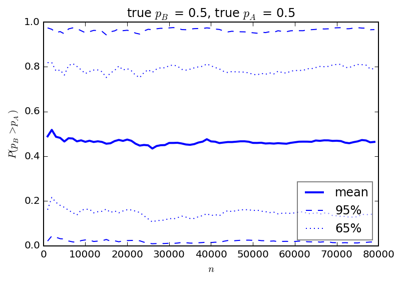
POI with equal probabilities for each group

The simulations show that nearly any POI can be observed when the two procedures truly have the same effect. Judging solely on POI, there is a decent chance that one could observe \(p_B\) to be greater than \(p_A\) when in fact it is not. What is surprising to me is that the spread of results never narrows. Running a longer test wont reduce the chance that a high POI will be reported.

How much better is the new procedure?

So POI isn't a great metric to base decisions on. Instead, I will use the expected gain to evaluate our results as described in a blog post by Chris Stuccio. Note that the referenced article actually considers the expected loss. Again I am interested in calculating how much better the new procedure is from the baseline, not whether it is worse, so I'll work with the expected gain. Again, the difference is in the order of the B and A labels in the expressions below.

The expected gain extends the concept of POI to not only include the probability that one outcome is better than the other, but also how much better the outcome will be. The metric is defined as \(P\left(\mathrm{max}\left[p_B - p_A, 0\right]\right)\)

\begin{align}P\left(\mathrm{max}\left[p_B-p_A,0\right]\right)&=\int_{0}^{1}\int_{0}^{1}dp_{A}dp_{B}\mathrm{max}\left[\left(p_{B}-p_{A}\right),\,0\right]\frac{p_{A}^{\alpha'_{A}-1}(1-p_{A})^{\beta'_{A}-1}}{\mathrm{B}(\alpha'_{A},\beta'_{A})}\frac{p_{B}^{\alpha'_{B}-1}(1-p_{B})^{\beta'_{B}-1}}{\mathrm{B}(\alpha'_{B},\beta'_{B})}\\ &=\int_{0}^{1}\int_{p_{A}}^{1}dp_{A}dp_{B}\left(p_{B}-p_{A}\right)\frac{p_{A}^{\alpha'_{A}-1}(1-p_{A})^{\beta'_{A}-1}}{\mathrm{B}(\alpha'_{A},\beta'_{A})}\frac{p_{B}^{\alpha'_{B}-1}(1-p_{B})^{\beta'_{B}-1}}{\mathrm{B}(\alpha'_{B},\beta'_{B})}\\ &=\frac{\mathrm{B}(\alpha'_{B}+1,\beta'_{B})}{\mathrm{B}(\alpha'_{B},\beta'_{B})}h(\alpha'_{A},\beta'_{A},\alpha'_{B}+1,\beta'_{B})-\frac{\mathrm{B}(\alpha'_{A}+1,\beta'_{A})}{\mathrm{B}(\alpha'_{A},\beta'_{A})}h(\alpha'_{A}+1,\beta'_{A},\alpha'_{B},\beta'_{B})\\ &=\frac{\alpha'_{B}}{\alpha'_{B}+\beta'_{B}}h(\alpha'_{A},\beta'_{A},\alpha'_{B}+1,\beta'_{B})-\frac{\alpha'_{A}}{\alpha'_{A}+\beta'_{A}}h(\alpha'_{A}+1,\beta'_{A},\alpha'_{B},\beta'_{B})\end{align}

where I have used the property of the Beta function

\begin{equation}\mathrm{B}\left(\alpha+1,\beta\right)=\mathrm{B}\left(\alpha,\beta\right)\frac{\alpha}{\alpha+\beta}.\end{equation}

The expected gain can be used to evaluate the outcome of an experiment. When reporting to decision makers, this outcome not only says that B turned out better than A, but it also provides an estimate of how much better it is.

What happens to the expected gain when the true values of \(p_B\) and \(p_A\) are equal? The POI wasn't always reliable in this situation. Is the gain a better metric? I'll turn again to simulated experimental results to find out.

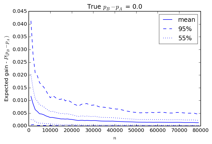
Expected gain with equal probabilities for each group

It's clear that the gain behaves much better than the POI did above. The gain quickly falls to a small value relatively quickly, and drops closer to the true value of 0 as the experiment continues. When looking for, say, a 1% gain from a new procedure, this metric would rightly indicate that such a gain was not likely.

On "peeking" and uncertainty in the gain

It has been suggested that one can "peek" at the gain throughout the experiment to watch for it to go above some threshold value, but this post by David Robinson shows through a series of simulations that this practice leads to an excessive rate of false positives (although the excessive false positive rate is not as extreme as if one were peeking at a p-value).

I'll give an example. Say we are running an experiment and are interested in implementing a new procedure (applied to group B) if we find a 1% gain in \(p_B\) over \(p_A\). But let's imagine that \(p_B\) is actually 1% lower than \(p_A\).

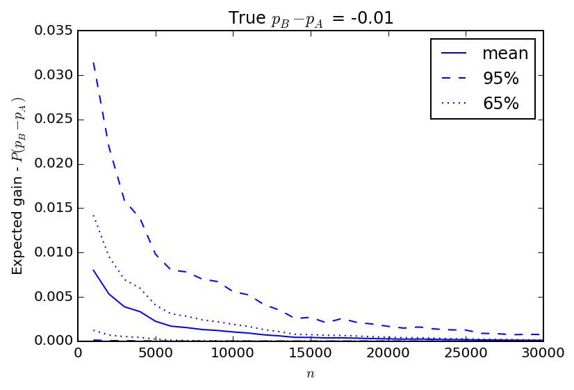
Gain as a function of experiment length when B is worse than A.

The figure above shows the expected gain from 100 simulated experiments where again I "peek" at the gain every 1000 trials. Until about 5000 trials there is a good chance that a 1% gain in B over A can be observed, and if I saw that and decided to stop the experiment early declaring success I would be making a mistake. The longer the experiment, the less likely it is that such a mistake would be made. But if I were watching the data to see a 1% gain and stopped the experiment as soon as I did, I would end up making a lot of bad decisions.

In the simulated examples above it is clear that with limited data, the variance in the observed expected gain in repeated experiments is too large and as a result reasonable decisions can't be made. How does one know when the result is "significant"? If the variance was known to be large and therefore the estimate of expected gain was inaccurate, then it would be obvious that more data was needed. Simulations can provide estimates of the variance, as above, but the variance in \(\mathrm{max}\left[p_B - p_A, 0\right]=\delta_{BA}\) can also be calculated directly

\begin{equation}P\left[\left(\delta_{BA}-\bar{\delta}_{BA}\right)^{2}\right]=\int_{0}^{1}\int_{p_{A}}^{1}dp_{A}dp_{B}\left(p_{B}-p_{A}-\bar{\delta}_{BA}\right)^{2}\frac{p_{A}^{\alpha'_{A}-1}(1-p_{A})^{\beta'_{A}-1}}{\mathrm{B}(\alpha'_{A},\beta'_{A})}\frac{p_{B}^{\alpha'_{B}-1}(1-p_{B})^{\beta'_{B}-1}}{\mathrm{B}(\alpha'_{B},\beta'_{B})}\end{equation}

The derivation proceeds very similarly to that of the expected gain

\begin{align}P\left[\left(\delta_{BA}-\bar{\delta}_{BA}\right)^{2}\right]=&\frac{\alpha'_{B}\left(\alpha'_{B}+1\right)}{\left(\alpha'_{B}+\beta'_{B}\right)\left(\alpha'_{B}+\beta'_{B}+1\right)}h(\alpha'_{A},\beta'_{A},\alpha'_{B}+2,\beta'_{B})\ldots\notag\\ &+\frac{\alpha'_{A}\left(\alpha'_{A}+1\right)}{\left(\alpha'_{A}+\beta'_{A}\right)\left(\alpha'_{A}+\beta'_{A}+1\right)}h(\alpha'_{A}+2,\beta'_{A},\alpha'_{B},\beta'_{B})\ldots\notag\\ &+\bar{\delta}_{BA}^{2}h(\alpha'_{A},\beta'_{A},\alpha'_{B},\beta'_{B})-2\frac{\alpha'_{A}}{\alpha'_{A}+\beta'_{A}}\frac{\alpha'_{B}}{\alpha'_{B}+\beta'_{B}}h(\alpha'_{A}+1,\beta'_{A},\alpha'_{B}+1,\beta'_{B})\ldots\notag\\ &+2\bar{\delta}_{BA}\frac{\alpha'_{A}}{\alpha'_{A}+\beta'_{A}}h(\alpha'_{A}+1,\beta'_{A},\alpha'_{B},\beta'_{B})-2\bar{\delta}_{BA}\frac{\alpha'_{B}}{\alpha'_{B}+\beta'_{B}}h(\alpha'_{A},\beta'_{A},\alpha'_{B}+1,\beta'_{B}).\end{align}

The expected gain, together with it's variance given here, are well suited to evaluating the experimental outcome. As an experiment is run the expected gain and it's variance can be calculated. If the gain is found to be significant relative to the square root of the variance, then the experiment can safely be stopped.

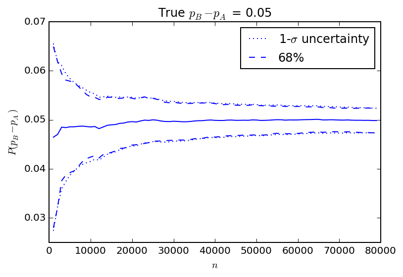
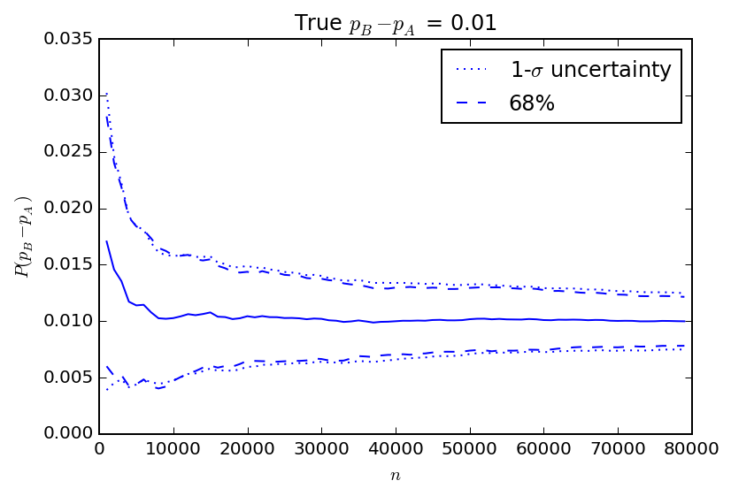
Average gain together with uncertainty compared to variance observed in experiments with 5% gain.

In the figure above, I show the results of another set of 100 simulations. In this case the true value of \(p_B\) is 5% higher than \(p_A\). The average of all observed gains converges on the correct difference pretty quickly. I also show the observed spread in gains over the 100 simulations as the interval covering 68% of the observed values and the 1-\(\sigma\) uncertainty as estimated by the square root of the variance calculated using the equation above. The closed form "1-\(\sigma\)" uncertainty calculation matches the spread of simulated results very closely. The figure below is similar, but for a true \(p_B\) that is only 1% higher than \(p_A\) for comparison.

Average gain together with uncertainty compared to variance observed in experiments with 1% gain.

What's the difference?

Thanks to Niels Oppermann for motivating this section.

The expected gain and its variance have both been calculated under the condition that \(p_B>p_A\). Instead, one could simply calculate the expected difference \(p_B-p_A=\delta'_{BA}\) without specifying that the new procedure outperforms the standard procedure

\begin{align}P\left(p_B-p_A\right)&=\int_{0}^{1}\int_{0}^{1}dp_{A}dp_{B}\left(p_{B}-p_{A}\right)\frac{p_{A}^{\alpha'_{A}-1}(1-p_{A})^{\beta'_{A}-1}}{\mathrm{B}(\alpha'_{A},\beta'_{A})}\frac{p_{B}^{\alpha'_{B}-1}(1-p_{B})^{\beta'_{B}-1}}{\mathrm{B}(\alpha'_{B},\beta'_{B})}\notag\\ &=\frac{\mathrm{B}(\alpha'_{B}+1,\beta'_{B})}{\mathrm{B}(\alpha'_{B},\beta'_{B})}-\frac{\mathrm{B}(\alpha'_{A}+1,\beta'_{A})}{\mathrm{B}(\alpha'_{A},\beta'_{A})}\notag\\ &=\frac{\alpha'_{B}}{\alpha'_{B}+\beta'_{B}}-\frac{\alpha'_{A}}{\alpha'_{A}+\beta'_{A}}\label{eq:exp_diff}\\ &=\bar{\delta}'_{BA}\label{eq:exp_diff2}\end{align}

This is just the difference between the posterior means for \(p_B\) and \(p_A\) as one might intuitively expect. What about the variance? The derivation is similar to the variance in the gain and the result is similar except a bit cleaner without the \(h(\alpha_A, \beta_A, \alpha_B, \beta_B)\) terms.

\begin{align}P\left[\left(\delta'_{BA}-\bar{\delta}'_{BA}\right)^{2}\right]=&\frac{\alpha'_{B}\left(\alpha'_{B}+1\right)}{\left(\alpha'_{B}+\beta'_{B}\right)\left(\alpha'_{B}+\beta'_{B}+1\right)}+\frac{\alpha'_{A}\left(\alpha'_{A}+1\right)}{\left(\alpha'_{A}+\beta'_{A}\right)\left(\alpha'_{A}+\beta'_{A}+1\right)}\ldots\notag\\ &-2\frac{\alpha'_{A}}{\alpha'_{A}+\beta'_{A}}\frac{\alpha'_{B}}{\alpha'_{B}+\beta'_{B}}-\bar{\delta}_{BA}^{2}.\label{eq:var_diff}\end{align}

The variance in the expected difference consists of the sum of two terms that are very nearly - but interestingly not quite - the posterior variances of \(p_B\) and \(p_A\) minus the square of the expected difference and a cross term.

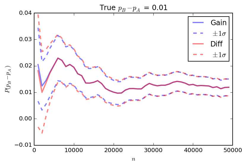
In the figure below I show a comparison of the expected difference and gain for a single simulated experiment including the "\(1\sigma\)" uncertainties (i.e. plus or minus the square root of the variance in each measure). In this case the true difference between \(p_B\) and \(p_A\) is 1%. After about 5000 trials, the two measures are essentially the same.

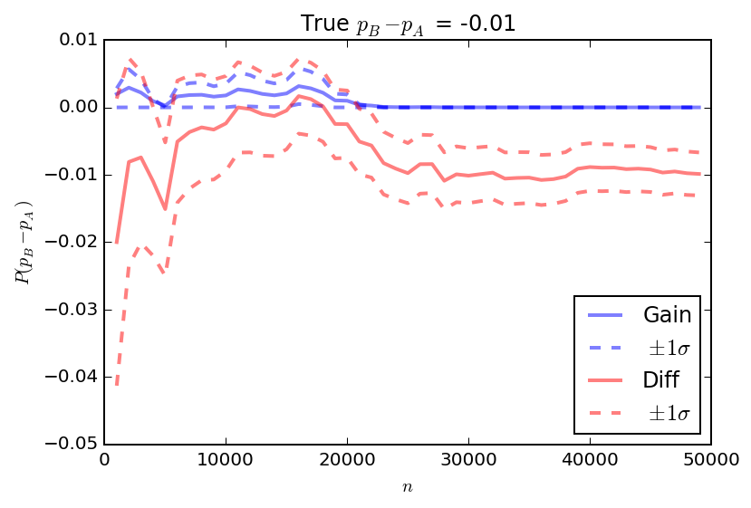
Comparison of expected gain and difference for a simulated example.

When the gain or difference is larger, the two quantities converge even more quickly. But what about when the difference is negative? In this case, there is much more discrepancy between the gain and the difference because the gain is a strictly positive quantity while the difference can take both positive and negative values.

Comparison of expected gain and difference for a simulated example with negative difference.

While I started by providing the gain and it's variance to build on the work of the blog posts of Miller and Stuccio, I will actually opt to use the expected difference and it's variance in my experiments.

Conclusions

So finally I have everything that I'll need to run basic experiments in situations with binary outcomes. The expected difference (eq.\(\,\ref{eq:exp_diff3}\)), together with it's variance (eq.\(\,\ref{eq:var_diff}\)), are enough to indicate not only how much better one might do by switching to a new procedure, but also how much one should trust the result. Experimental results can be monitored regularly as long as both the difference and variance are evaluated at each step, and it's fine to stop the experiment if the difference is found to be good enough when compared to the uncertainty.

These results apply to two procedure (A/B) tests where outcomes are binary. Similar results can be obtained when testing 3 or more procedures in parallel or if the outcomes are not binary but e.g. counts or rates instead. For example, Evan Miller calculates POI for count data and for three test groups. An expected difference and it's variance could be calculated in these cases as well.